Modeling of Type 1 Wind Turbine Generators

Author: National Renewable Energy Laboratory^[1]

While there are many wind turbine dynamic models available in the literature, the focus is largely on modeling variable-speed wind turbines. These models often oversimplify the mechanical drive train and aerodynamics, since the aim is to evaluate power and rotor speed control mechanisms. Thus, there exists a gap in the literature which the model described in this chapter attempts to address. While the model’s central purpose is to study the interaction between the wind turbine and the power system, it may also be used to examine the interaction of aerodynamic, mechanical, and electrical functions within the wind turbine. This model is a platform on which more advanced variable-speed wind turbine models can be developed. The complete model has been implemented in PSCAD/EMTDC for the purposes of this article. However, the model is straightforward to implement using other popular simulation packages such as MATLAB/Simulink. The model is based on parameters from a NEG Micon 1.5-MW turbine.

Background

Turbine Properties
Turbine make	NEG Micon NM72C 1.5MW
Regulation method	Active stall (disabled)
Rotor diameter	72 m
Hub height	62 m or 78 m
Number of blades	3
Cut-in wind speed	4 m/s
Cut-out wind speed	20 m/s
Rated wind speed	13 m/s
Rotor speed	17.3 rpm

Wind turbines are designed to capture the kinetic energy present in wind and convert it to electrical energy. An analogy can be drawn between wind turbines and conventional generating units which harness the kinetic energy of steam. From a modeling standpoint, a fixed-speed wind turbine consists of the following components:

• Turbine rotor and blade assembly (prime mover);
• Shaft and gearbox unit (drivetrain and speed changer);
• Induction generator;
• Control system.

The interaction between each of the components listed above determines how much kinetic energy is extracted from the wind. Modeling of the electrical subsystems is fairly straightforward, as power system modeling software usually includes a built-in induction machine model. However, modeling of the aerodynamics and mechanical drivetrain is more challenging. These components are modeled based on the differential and algebraic equations that describe their operation. The following sub-sections describe the modeling of the components listed above.

Aerodynamic Block

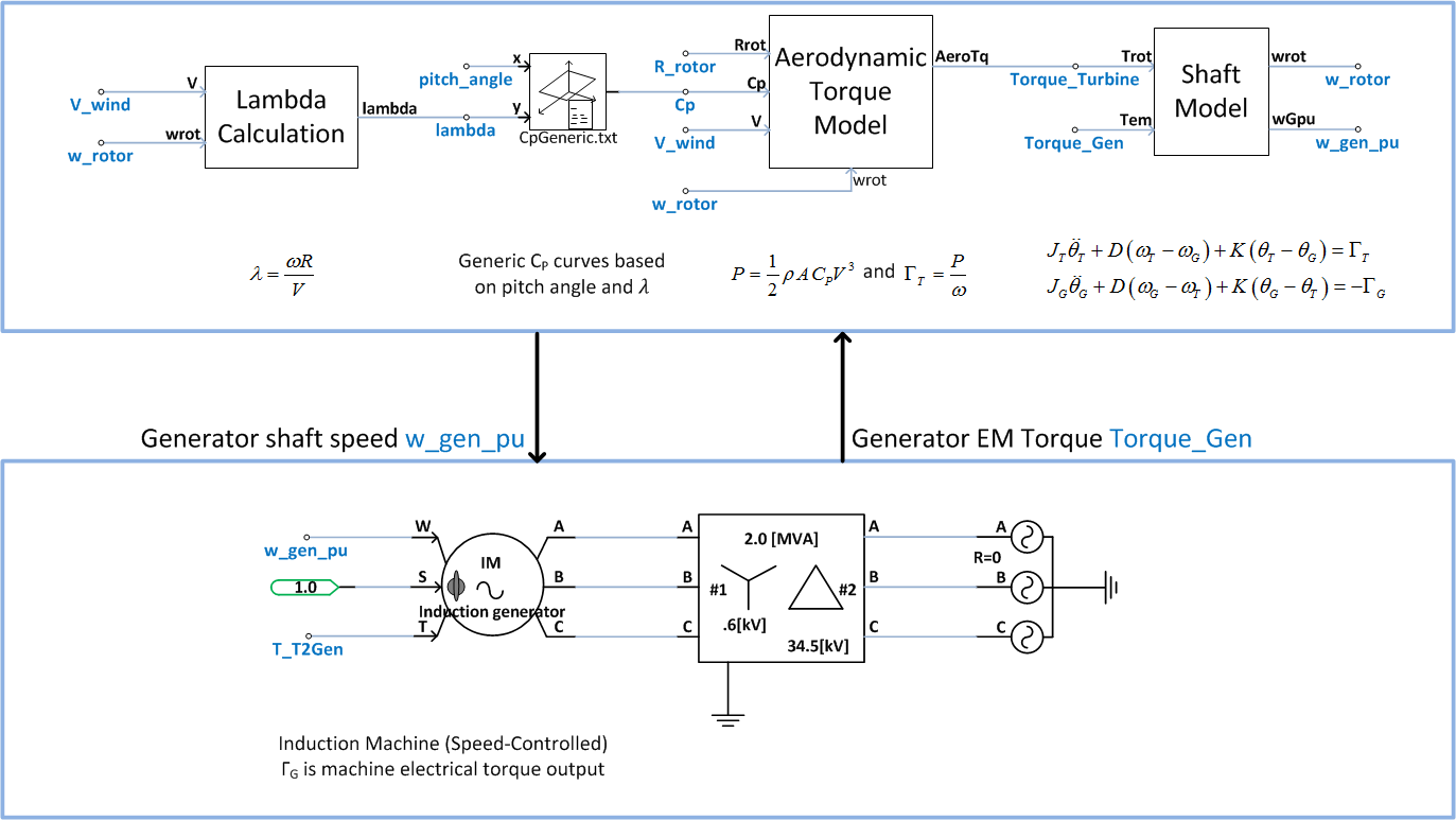
The aerodynamic block consists of three subsystems: tip-speed ratio calculation, rotor power coefficient (C_P) calculation, and aerodynamic torque calculation. Wind speed and pitch angle are user-defined inputs. Since the model is intended to study the dynamic response of wind turbines to grid events, the assumption is usually made that the wind speed stays constant during the grid event. However, this model allows the wind speed input signal to be set to any value at the start of the simulation run-time and also to be modified during the run. It is also possible to use a time-series of actual wind speed data. Since the focus of this article is on a fixed-speed stall-regulated wind turbine model, the pitch angle is fixed at the start of the simulation so that the wind turbine achieves rated power at the rated wind speed.

Tip-Speed Ratio Calculations

The tip-speed ratio or TSR, denoted by λ, is the ratio of the blade-tip linear speed to the wind speed^[2]. The TSR determines the fraction of available power extracted from the wind by the wind turbine rotor. In a fixed-speed wind turbine, the blade tip speed is held relatively constant since the rotor is connected directly to the induction generator via a gearbox, and the induction generator is directly connected to the grid. The TSR can be calculated as follows

\(\lambda=\frac{\omega_{rotor} · R_{rotor}}{V_{wind}}\)

where,
ω_rotor = rotor angular speed [rad/s]
R_rotor = rotor radius [m]
V_wind = wind speed [m/s]

Rotor Power Coefficient (C_p) Calculation

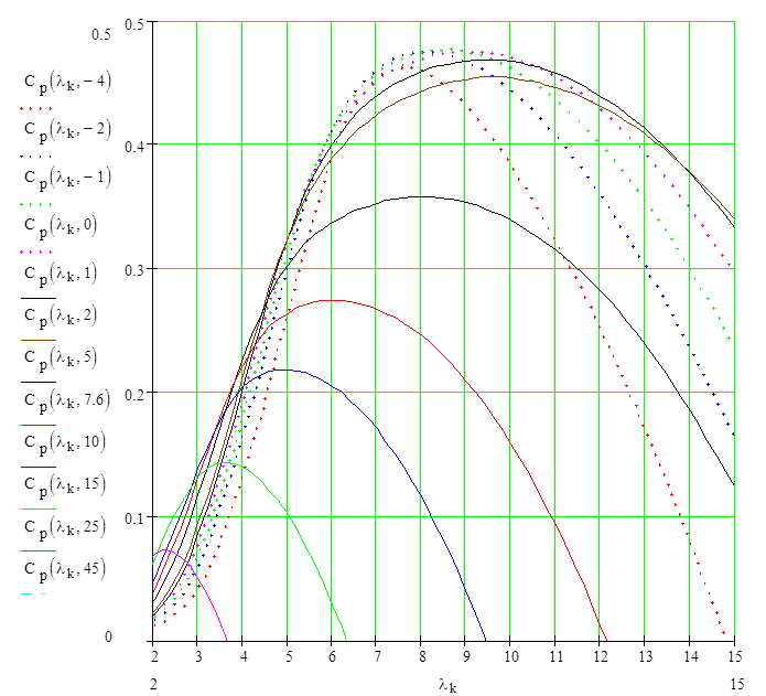
The TSR, together with the user-defined blade pitch angle β, are used to calculate the rotor power coefficient, denoted by C_P. The rotor power coefficient is a measure of the rotor efficiency and is defined as

\(\mathrm{C}_P=\frac{Extracted\ Power}{Power\ in\ Wind}=\frac{P_{rotor}}{P_{wind}}\)

There is a constant value of λ which, if maintained for all wind speeds, will result in an optimal C_P curve and optimal power extraction from the wind. Variable-speed wind turbines are equipped with a pitch-change mechanism to adjust the blade pitch angle and obtain a better power coefficient profile.
In case of a fixed-speed wind turbine which is directly connected to the grid, the electrical generator speed, ω_gen, is essentially fixed by the grid frequency. In turn, the rotor speed, ω_rot, is also fixed since it is directly connected to the generator via a gearbox. As a result, the blade tip speed is practically unchanged. As the wind speed increases, the C_P of a direct-connect fixed-speed wind turbine will increase at first, achieve an optimal value at rated wind speed (the wind speed corresponding to rated power output), and decrease at higher wind speeds. In the model, a set of generic C_P curves are used to calculate the value of C_P^[3].

Aerodynamic Torque Calculation

The kinetic energy E (in J) of an air mass m (in kg) moving at a speed V_wind (in m/s) is given by:

\(E=\frac{1}{2}mV_{wind}^2\)

If the air density is ρ (kg/m³), mass flow through an area A is given by:

\(\dot{m}=ρAV_{wind}\)

Thus, an equation for the power (in W) through a cross-sectional area A normal to the wind is:

\(P_{wind}=\frac{1}{2}ρAV_{wind}^3\)

In the case of a wind turbine, area A is the area swept by the rotor blades. Only a part of this power may be captured due to the non-ideal nature of the rotor, hence the need for the coefficient C_P.:

\(P_{rotor}=\frac{1}{2}ρ\cdot\mathrm{C}_p\cdotπ\cdot\mathrm{R}_{rotor}^2\cdot\mathrm{V}_{wind}^3\)

The aerodynamic torque developed (in Nm) can then be calculated:

\(\Gamma_{rotor}=\frac{P_{rotor}}{ω_{rotor}}=\frac{\frac{1}{2}\cdotρ\cdot\mathrm{C}_p\cdotπ\cdot\mathrm{R}_{rotor}^2\cdot\mathrm{V}_{wind}^3}{ω_{rotor}}\)

Mechanical Drive-Train

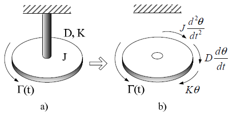
The mechanical block consists of the rotor shaft, generator shaft, and a gearbox. The shafts and the gearbox are modeled using a two-mass inertia representation. For a rotational system^[4], consisting of a disk with a moment of inertia J mounted on a shaft fixed at one end, let us assume that the viscous friction coefficient (damping) is D and that the shaft torsional spring constant (stiffness) is K. The torque acting on the disk can be calculated from the free-body diagram of the disk, as follows

\(\Gamma(t)=J\frac{d^2\theta(t)}{dt^2}+D\frac{d\theta(t)}{dt}+K\theta(t)\)

A more complex rotational system consists of two such systems. The two systems are coupled through a gear train, and Γ is the external torque applied to the disk of System 1. Γ₁, Γ₂ are transmitted torques. N₁, N₂ are the numbers of teeth of Gear 1 and Gear 2. J₁, J₂, D₁, D₂, K₁, K₂ are the moments of inertia, damping, and stiffness of System 1 and System 2, respectively. The system is still time-dependent, but the notation t is dropped for the sake of clarity.

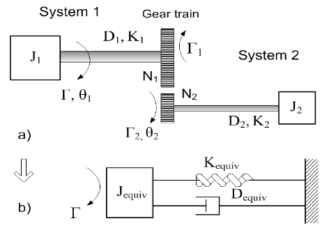
The torque equation at J₁ can then be calculated as:

\(\Gamma_1=J_1\frac{d^2\theta_1}{dt^2}+D_1\frac{d\theta_1}{dt}+K_1\theta_1\)

The torque equation at J₂ can then be calculated as:

\(\Gamma_2=J_2\frac{d^2\theta_2}{dt^2}+D_2\frac{d\theta_2}{dt}+K_2\theta_2\)

Since Γ₁ = (N1/N2)Γ₂ and Θ₂ = (N1/N2)Θ₁, the quantities on Gear 2 side can be referred to the Gear 1 side.:

\(\Gamma_1=\left (\frac{N_1}{N_2} \right)\left (J_2\frac{d^2\theta_2}{dt^2}+D_2\frac{d\theta_2}{dt}+K_2\theta_2 \right)\) \(\Gamma_1=\left (\frac{N_1}{N_2} \right)\left [J_2\left (\frac{N_1}{N_2} \right)\frac{d^2\theta_1}{dt^2}+D_2\left (\frac{N_1}{N_2} \right)\frac{d\theta_1}{dt}+K_2\left (\frac{N_1}{N_2} \right)\theta_1 \right]\) \(\Gamma_1=J_{refl}\frac{d^2\theta_1}{dt^2}+D_{refl}\frac{d\theta_1}{dt}+K_{refl}\theta_1\)

where J_refl, D_refl, and K_refl are the quantities reflected on the Gear 1 side. Substituting the above equations and rearranging them, we obtain the equation for the applied torque. The gear train is eliminated in the equivalent system.:

\(\Gamma=J_{equiv}\frac{d^2\theta_1}{dt^2}+D_{equiv}\frac{d\theta_1}{dt}+K_{equiv}\theta_1\)

where,

\(J_{equiv}=J_1+J_2\left (\frac{N_1}{N_2} \right)^2=J_1+J_{refl}\)

 

\(D_{equiv}=D_1+D_2\left (\frac{N_1}{N_2} \right)^2=D_1+D_{refl}\)

 

\(K_{equiv}=K_1+K_2\left (\frac{N_1}{N_2} \right)^2=K_1+K_{refl}\)

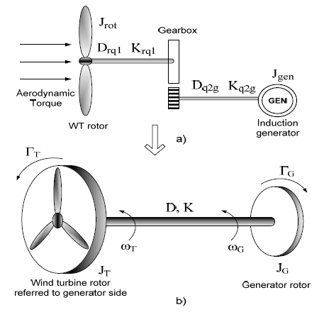
The wind turbine drive-train can therefore be modeled as a two-mass system coupled through a gear train. The quantities on the wind turbine rotor side of the gearbox can be reflected to the generator side. This eliminates the gear ratio and results in a two-mass representation of the wind turbine. Neglecting the effects of the gearbox moment of inertia, damping, and stiffness is justifiable since the moment of inertia of the wind turbine rotor is comparatively very high.
Torque equations representing the mechanical behavior of the wind turbine are derived, based on the two-mass model. The aerodynamic torque from the wind turbine rotor and the electromechanical torque from the direct-connect induction generator act in opposition to each other. Torque equations with all quantities referred to the generator side are

\(J_T\ddot {\theta_T}+D(ω_T-ω_G)+K(\theta_T-\theta_G)=\Gamma_T\) \(J_G\ddot {\theta_G}+D(ω_G-ω_T)+K(\theta_G-\theta_T)=-\Gamma_G\)

where,
J_T, J_G = moments of inertia of the wind turbine rotor and the generator [kgmm]
Γ_T, Γ_G = wind turbine aerodynamic and generator electromagnetic torque [Nm]
ω_T, ω_G = wind turbine rotor and the generator speed [rad/s]
Θ_T, Θ_G = angular position of the rotor and the generator [rad]
D, K = equivalent damping and stiffness [Nms/rad], [Nm/rad]
Speeds and torques of the turbine rotor and the generator can be determined for each simulation time step by solving the above equations using a state-space approach. The state-space equations are

\(\frac{d}{dt}(\theta_G-\theta_T)=(ω_T-ω_G)\)
\(\dot {\omega_T}=\left (\frac{1}{J_T} \right)\left [\Gamma_T-D(\omega_T-\omega_G)-K(\theta_T-\theta_G) \right]\)
\(\dot {\omega_G}=\left (\frac{1}{J_G} \right)\left [D(\omega_T-\omega_G)+K(\theta_T-\theta_G)-\Gamma_G \right]\)

Induction Generator

Most fixed-speed wind turbines employ squirrel-cage induction machines, for which models are readily available in most power system modeling software. The platform of choice to implement the model was PSCAD/EMTDC, and the in-built induction machine model was used. Alternatively, if the modeling platform does not offer a built-in model, users may develop third- or fifth-order algebraic models for induction machines based on the literature available^[5].

Induction generator ratings
Rated MVA	1.5 MVA
Rated Voltage	0.69 kV line-to-line
Number of poles	6
Rated frequency	60 Hz
Stator/rotor turns ratio	0.379
Induction generator parameters
Stator winding resistance	0.0047 pu
Squirrel-cage resistance	0.0021 pu
Stator leakage inductance	0.08 pu
Squirrel-cage inductance	0.0478 pu
Magnetizing inductance	6.8 pu
Angular moment of inertia	0.578 s

Control Block

Because the focus of the modelling exercise is a fixed-speed wind turbine, pitch-angle control and power control are absent. This block may be added later for modelling variable-speed wind turbines or for reactive power management.

Complete Model Implemented in PSCAD/EMTDC

The complete model, implemented in PSCAD/EMTDC, is connected to an ideal voltage source (representing the grid) through a step-up transformer.

Power Curve for Fixed-Speed Model

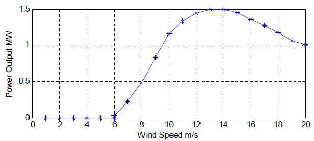
The most fundamental measure of a wind turbine’s performance is given by its power curve. The wind turbine model developed here is tested by running the simulation at wind speeds from 1 to 20 m/s, with increments of 1 m/s between runs. As expected, the power output peaks at rated wind speed and then falls due to stalling.

Data for Power Curve
Vwind (m/s)	Pout (MW)
6	0.03
7	0.22
8	0.484
9	0.825
10	1.159
11	1.332
12	1.441
13	1.5
14	1.5
15	1.452
16	1.359
17	1.267
18	1.171
19	1.063
20	1.007

 

Dynamic Response

To demonstrate the model’s ability to reproduce wind turbine dynamics, a test was created. The wind turbine was operated with a constant wind speed (13 m/s). This wind speed was chosen to be the rated value. A voltage sag on the grid was simulated, and the real and reactive power response of the wind turbine was observed. Note that this is not an implementation of low-voltage ride through (LVRT), but rather a test of dynamic response. The grid voltage drops from 1 p.u. to 0.8 p.u. at t=15s, and the sag persists for 18 cycles (0.3 seconds). The intent of the test is to show that the model does indeed respond to events occurring in the dynamic timescale and that the response of the machine to this event is realistic.

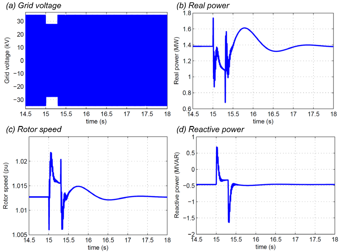
As expected, the step changes in the grid voltage magnitude when the sag begins and ends cause an immediate response. Note that the speed does not change by much (approximately 2%), as expected from a fixed-speed wind turbine. The real power and reactive power outputs experience a disturbance too, and the outputs show that a mechanical oscillation occurs after the sag ends, and that the oscillation eventually damps out.

References

- ↑ NREL, Dynamic Models for Wind Turbines and Wind Power Plants (NREL/SR-5500-52780), October 2011, [Online]. Available: http://www.nrel.gov/docs/fy12osti/52780.pdf. [Accessed February 2013].
- ↑ 2.0 2.1 J. Manwell and J. McGowan, Wind energy explained: theory, design and application. Wiley Chichester, 2003.
- ↑ R. Delmerico, N. Miller, W. Price, and J. Sanchez-Gasca, “Dynamic Modeling of GE 1.5 and 3.6 MW Wind Turbine-Generators for Stability Simulations,” in IEEE Power Engineering Society General Meeting, (Toronto, ON).
- ↑ 4.0 4.1 B. Kuo, Automatic control systems. Prentice Hall, 1995.
- ↑ V. Akhmatov, Induction generators for wind power. Paul & Co. Pub. Consortium, 2007.