Validation of Simulated Irradiance and Power

Author: Sandia National Laboratories^[1]

The Western Wind and Solar Integration Study (WWSIS) Phase II seeks to quantify the effects on thermal generation plants that may result from integration onto the transmission network of variable generation sources, including wind and solar power plants. The study assumes a large number of additional generating resources, including utility-scale photovoltaic (PV), concentrating solar power (CSP) plants, distributed PV, and wind generation, are added to the grid. Power balance simulations are performed for a study period of one year to quantify the operating costs associated with the additional levels of variable generation.

For the WWSIS Phase II study, time series of power output from hypothetical solar plants were calculated from simulated time series of one-minute irradiance at each plant’s location. For all types of solar power, the key input to these calculations is the time series of irradiance at one-minute time steps for calendar year 2006 averaged over the spatial extent of each hypothetical solar plant. Measurements of irradiance at with this temporal and spatial resolution are not available. National Renewable Energy Laboratory staff devised methods to simulate the required irradiance.

To build confidence in the conclusions of this study, Sandia National Laboratories conducted validation of the algorithm used to simulate irradiance, and performed a qualitative review of the methods that calculate power from irradiance. We concluded that the simulated power output from utility-scale solar plants was reasonable for the purposes of the WWSIS Phase II study.

Introduction

The Western Wind and Solar Integration Study Phase II

The Western Wind and Solar Integration Study (WWSIS) Phase II began in March 2011. This study seeks to quantify the effects (e.g., costs associated with cycling and ramping) on thermal generation plants that may result from integration onto the transmission network of variable generation sources, including wind and solar power plants.

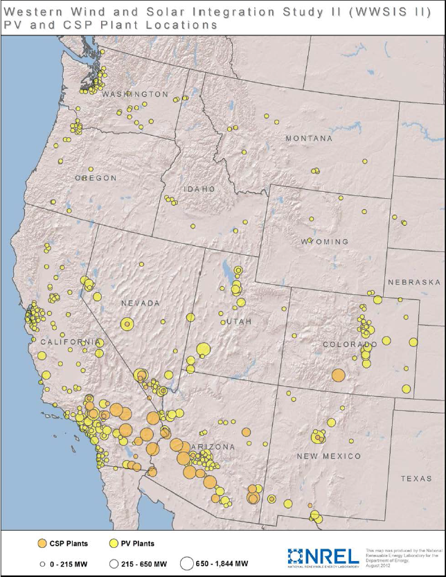
Figure on the right illustrates the distribution of utility-scale PV and CPV plants assumed for the WWSIS study. The majority of solar power capacity is assumed to be located in southwest Arizona, southern Nevada, southwest Utah and southern California, with smaller but significant concentrations near large urban areas within the western United States, e.g., near the Front Range in Colorado, central New Mexico, Salt Lake City, Utah, the San Francisco bay area in California and Seattle, WA.

The required inputs for the study include irradiance at one-minute time steps for calendar year 2006 averaged over the spatial extent of each hypothetical solar power facility. Measurements of irradiance at this temporal and spatial resolution are not available. Irradiance measurements with ground-based sensors are available at one-minute time resolutions for a few locations within the study area. In place of direct measurement, irradiance may be calculated from satellite images covering the entire study area; however, the irradiance thus obtained is generally at 60-minute time intervals and at 10 km grid spacing.

National Renewable Energy Laboratory (NREL) staff has developed a simulation method to generate one-minute time series of global horizontal irradiance (GHI) and direct normal irradiance (DNI) in each grid cell of a 10 km grid covering the study area. Irradiance is considered spatially uniform within a grid cell. Simulated irradiance is used with recorded air temperature and general characteristics of the hypothetical solar power systems to estimate power from each power system at one-minute intervals for the study period.

The simulation method uses available satellite imagery to estimate a spatial average GHI for each hour of the year at each grid cell as the spatial average over the area around the cell, along with a variability category for each hour that is determined by the variation in the satellite image in the area. For the WWSIS, spatial fields of GHI are obtained from the SolarAnywhere® data set^[2]. Separately, a set of statistics describing properties of one-minute time series of clear-sky index (i.e., GHI divided by clear-sky GHI) is derived from a collection of measurements of GHI at a few locations within the study area. For each hour, the spatial average GHI and variability category (determined from satellite imagery) are used to select statistics; the statistics are used in turn to stochastically generate one-minute clear-sky index values for that hour. Clear-sky index is then multiplied by clear-sky GHI irradiance to obtain GHI and DNI is in turn derived from GHI. The algorithm is described in a forthcoming NREL report^[3].

Irradiance simulations were parameterized using data recorded generally at one-minute intervals at a number of locations that generally (but not comprehensively) represent the assumed concentrations of solar power systems. Data were taken from an archive (MIDC) maintained by National Renewable Energy Laboratory^[4].

Sites With Data Used to Parameterize Irradiance Simulation

Location	Latitude	Longitude	Years when data were used
Solar Radiation Research Laboratory, Golden, CO	39.742	105.18	2005, 2006, 2007, 2009, 2010
National Wind Technology Center M2 Tower, Boulder, CO	39.91065	105.2348	2005, 2006, 2007, 2009, 2010
University of Nevada, Las Vegas, NV	36.06	115.08	2006, 2007, 2009, 2010
Nevada Power Clark Station, Las Vegas, NV	36.08581	115.0519	2006, 2007, 2009
Loyola Marymount University, University Hall, Los Angeles, CA	33.96667	118.4228	2009, 2010
Humboldt State University, Arcata, CA	40.880	124.080	2009
Sun Spot One, San Luis Valley, Alamosa, CO	37.561	106.0864	2009

Validation Approach

In a formal sense, no proof can be offered that the simulated irradiance reproduces, within some tolerance, the irradiance that occurred in 2006. Instead, we compare characteristics, such as cumulative distributions, of the simulation with those of measurements. Whether the simulation method and its results are valid is a qualitative judgment regarding the suitability of the data for its intended use in the WWSIS study. Our analysis seeks to inform this judgment.

This report documents a validation effort that considers both the simulated irradiance data sets as well as the method for calculating power. Our validation effort first examines the results of the irradiance simulation. To enable comparison between simulated irradiance and a larger set of measured irradiance than are available from 2006, the simulation algorithm was used to generate irradiance data for 2010. These simulated data for 2010 are compared to measured irradiance from a variety of sources. We make five primary comparisons between the simulated and measured irradiance:

1. We compare distributions of global horizontal irradiance (GHI), for both short (i.e, one and three- minute) time steps as well as for hourly average values. Agreement between simulated and measured GHI provides confidence that irradiance levels (and simulated power levels from hypothetical non-concentrating photovoltaic (PV) plants) occur as often as they appear in measurements.
2. We compare distributions of the rates of change in GHI (i.e., ramp rates) for both one minute and hourly changes. This comparison provides confidence that the variability in time series of GHI generated by the simulation is consistent with that observed in measurements, and consequently, that variability in power from non-concentrating PV plants is reasonably represented.
3. We compare the correlation between clear sky index values (i.e., irradiance divided by clear sky irradiance) at different locations as a function of distance between locations and time between observations. Agreement between correlation values for simulated and measured irradiance provides confidence that the simulations preserve spatial relationships evident in irradiance measurements. To confirm that correlations represent the level of agreement between the time series, we also examine the joint distribution of clear-sky index values for pairs of locations.
4. We compare the correlation between changes in clear-sky index values at different locations as a function of distance between locations and time between values. This comparison provides confidence that changes in irradiance at different locations reflect appropriate spatial relationships.
5. We compare distributions of direct normal irradiance (DNI) and of changes in DNI. Agreement in these comparisons provides confidence that power and variability in power from concentrating PV (CPV) plants are reasonably represented.

We also performed a qualitative technical review of the methods for determining PV and CPV system output from simulated irradiance and temperature. Our review focuses on the suitability of the modeled solar power system output for use in the WWSIS study, to wit:

1. Are the approaches used to model solar power systems consistent with accepted practices?
2. Do the modeled results appear qualitatively consistent with expectations?

We did not perform a review of methods for determining output of concentrating solar power (CSP) systems, as the relevant modeling methods are outside of our expertise. However, we believe that the comparison of GHI and DNI between simulations and measurements should be helpful to a review of CSP calculations.

Analysis of simulated irradiance

Locations Considered for Analysis

Our validation efforts focus on simulation results for locations assumed to have significant solar power production in the WWSIS study. Accordingly, we focus our validation on multiple sites in southern Arizona, Nevada and California, and consider fewer sites in New Mexico, Colorado, Utah and Washington. We make no attempt to validate simulated irradiance at other locations (e.g., eastern Oregon) which have only minor influence on the WWSIS study conclusions.

Table bellow summarizes the validation locations, which fall into three general categories:

1. Three sites (sites numbers 1 to 3) at which measured data for 2010 (as well as for other years) were used in the simulations. These sites include: the National Wind Technology Center M2 Tower near Boulder, CO; the Solar Radiation Research Laboratory near Golden, CO; and the University of Nevada, Las Vegas, NV. Validation at these sites confirms that the simulation can replicate characteristics of measured data for locations and years that were used to parameterize the distributions underlying generation of oneminute irradiance.
2. Three sites (site numbers 3 to 6) at which measured data for years other than 2010 were used in the simulations. These sites include: Sun Spot One, near Alamosa, CO; the Nevada Clark Power Station in Las Vegas, NV; and Loyola Marymount University in Los Angeles, CA. Validation at these sites confirms that the simulation can replicate characteristics of measured data at locations where data from earlier years were used to parameterize the distributions underlying generation of one-minute irradiance.
3. Twenty two sites (site numbers 7 through 28) at which measured data at various time resolutions are available and which were not used to parameterize the simulation.

Sites Used for Validation

Site Number	Site Name (data source1)	Latitude	Longitude	Validation category
1	National Wind Technology Center M2 Tower, Boulder, CO (MIDC)	39.91065	105.2348	Data for 2010 used to parameterize simulations. Validation confirms simulation can replicate measured data
2	Solar Radiation Research Laboratory, Golden, CO (MIDC)	39.742	105.18	Data for 2010 used to parameterize simulations. Validation confirms simulation can replicate measured data
3	University of Nevada, Las Vegas, NV (MIDC)	36.06	115.08	Data for 2010 used to parameterize simulations. Validation confirms simulation can replicate measured data
4	Sun Spot One, San Luis Valley, Alamosa, CO (MIDC)	37.561	106.0864	Data for years other than 2010 used to parameterize simulations. Validation confirms simulation based on earlier years can replicate measured data for later years
5	Nevada Power Clark Station, Las Vegas, NV (MIDC)	36.08581	115.0519	Data for years other than 2010 used to parameterize simulations. Validation confirms simulation based on earlier years can replicate measured data for later years
6	Loyola Marymount University, University Hall, Los Angeles, CA (MIDC)	33.96667	118.4228	Data for years other than 2010 used to parameterize simulations. Validation confirms simulation based on earlier years can replicate measured data for later years
7	3439 (proprietary)	32.861	115.638	Measured data at 1-minute resolution
8	3443 (proprietary)	34.566	117.694	Measured data at 1-minute resolution
9	3444 (proprietary)	35.018	118.118	Measured data at 1-minute resolution
10	4252 (proprietary)	32.952	113.491	Measured data at 1-minute resolution
11	4255 (proprietary)	35.79	114.969	Measured data at 1-minute resolution
12	4258 (proprietary)	33.42	114.749	Measured data at 1-minute resolution
13	ABQ, Albuquerque, NM (ISIS)	35.04	106.62	Measured data at 3-minute resolution
14	SLC, Salt Lake City, UT (ISIS)	40.77	111.97	Measured data at 3-minute resolution
15	HAN, Hanford, CA (ISIS)	36.31	119.63	Measured data at 3-minute resolution
16	SEA, Seattle, WA (ISIS)	47.68	122.25	Measured data at 3-minute resolution
17	BOU, Boulder, CO (Surfrad)	40.13	105.24	Measured data at 3-minute resolution
18	SMUD Anatolia, Sacramento, CA (MIDC)	38.54586	121.2403	Measured data at 1-minute resolution
19	Cedar City, UT (MIDC)	37.69601	113.1648	Measured data at 1-minute resolution
20	Bonita, AZ (AZMET)	32.46361	109.9294	Measured data at 1-hour resolution
21	Buckeye, AZ (AZMET)	33.4	112.6833	Measured data at 3-minute resolution
22	Marana, AZ (AZMET)	32.42235	111.1634	Measured data at 3-minute resolution
23	Maricopa, AZ (AZMET)	33.06861	111.9717	Measured data at 3-minute resolution
24	Mojave, AZ (AZMET)	34.96722	114.6058	Measured data at 3-minute resolution
25	Paloma, AZ (AZMET)	32.92667	112.8956	Measured data at 3-minute resolution
26	Phoenix Encanto, Phoenix, AZ (AZMET)	33.47917	112.0964	Measured data at 3-minute resolution
27	Phoenix Greenway, Phoenix, AZ (AZMET)	33.62139	112.1083	Measured data at 3-minute resolution
28	Yuma Valley, AZ (AZMET)	32.7125	114.705	Measured data at 3-minute resolution
1 ISIS: Integrated Surface Irradiance Study; Surfrad: Surface Radiation Budget Network; MIDC: Measurement and Instrumentation Data Center; AZMET: Arizona Meteorological Network;

Spatial and Temporal Resolution

Comparison between simulated and measured irradiance must take into account differences in spatial and temporal resolution. Measured data are all point values, averaged over the time interval (i.e., one minute, three minutes or one hour) between reported values. The spatial and temporal resolution of simulated irradiance results from the data from which the simulations are generated. The satellite-derived irradiance values, obtained every 30 minutes and for each 1 km² pixel in an image, represent instantaneous measurements of the aggregate irradiance over each pixel, i.e., spatial average irradiance at a point in time. These values are used as indices to select parameter values for the distributions used to generate the one-minute irradiance values; the parameter values are derived from time series of one-minute average irradiance measured at points on the ground. Consequently, we view the simulated irradiance values as one-minute averages at single points.

Comparison of Distributions of GHI

We compared the cumulative distribution functions (CDFs) of GHI between simulations and measurements, at the temporal resolution of each measurement. In all comparisons, the distributions were assembled from GHI values exceeding 30 W/m², to exclude times other than daylight hours. We examine the distributions for the entire year as well as for two-week periods within each season of the year, specifically, two-week periods beginning on February 1, May 1, August 1, and November 1.

Generally, we found that the simulation results:

• Agreed reasonably with measurements at locations where 1-minute or 3-minute data was available and which are not remote from sites used to parameterize the simulation;
• Agreed reasonably, but with an insignificant, consistent bias, at locations where only hourly average data is available;
• Showed significant disagreement at two locations remote from sites used to parameterize the simulation;
• Showed infrequent, non-physically large irradiance values. Within regions most important to the WWSIS study, we conclude that the simulation produces time series of GHI in which irradiance levels occur at frequencies consistent with those observed in measurements. At locations remote from those used to parameterize the simulation, we found significant disagreement between simulated and observed distributions of GHI.

At times, the simulation yields non-physically large values of GHI. If the algorithm (or its parameters) were improves to reduce the occurrence of these values, we believe that differences in the variability of simulated and measured GHI would also be reduced.

Locations Used to Parameterize the Simulation

The simulation method^[3] uses measured GHI at several locations to estimate a set of parametric distributions for one-minute clear-sky index. Sites 1 through 3 were among these locations. At these sites, measured data from 2010 was included when estimating the distributions. We compared simulation results to measured data at these sites, to confirm that the simulation reproduces measurements for time periods and locations where the simulation was effectively calibrated. We also compared simulations with measurements at locations where data from other years was used to estimate the distributions.

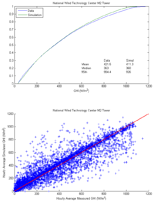
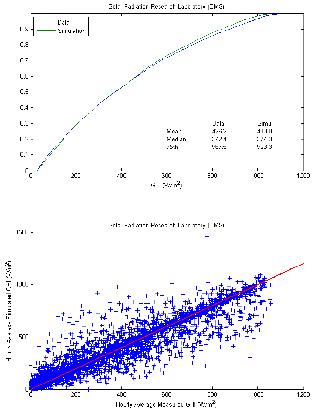
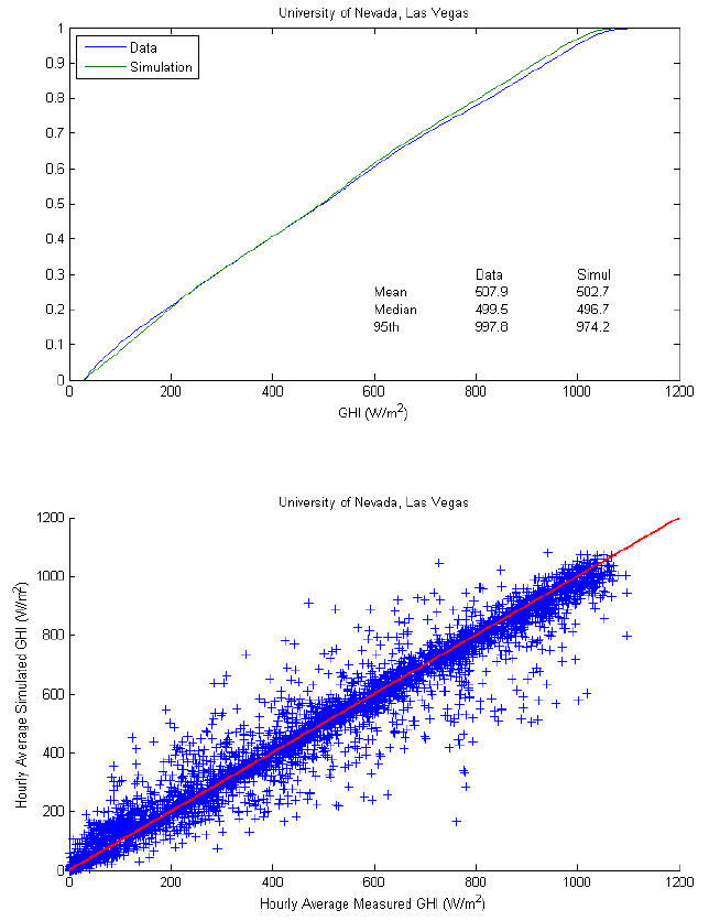
At sites 1 through 3, the simulation reasonably reproduced the distributions of GHI. Mean and median GHI are generally within 2% of measured values. The simulations somewhat understate the frequency at which the highest levels of GHI occur as indicated by lower values at the 95^th percentile of simulated GHI.

Comparison of synchronous hourly averaged GHI shows considerable scatter indicating that while the simulation produces distributions of GHI with acceptable statistics, it is less able to produce time series that replicate measurements. It is likely that the scatter in hourly averaged GHI is due in part to the different spatial scales involved in each hourly average value. Measurements are obtained at points. In contrast, one parameter to the algorithm that stochastically generates one-minute GHI is the hourly average irradiance obtained as a spatial average over an area of 100 km² on a satellite image. Comparison of variances of time series of hourly average GHI, between measured and simulated, confirms that simulated variance is lower, which we would expect if simulated GHI is affected by some level of spatial averaging that is not operating on measured GHI. Because the simulation’s output is passed through a filter intended to represent the averaging that occurs over the spatial extent of a power plant, the differences in variance are acceptable in the context of the WWSIS study.

However, the data underlying the scatterplot in figure on the right showed an undesirable feature of the simulation output: occasionally the simulation produces non-physically large GHI values, at times approaching 2000 W/m². While GHI exceeding clear-sky values have been observed (e.g.,^[5],^[6]) due to refraction from edges of passing clouds (termed cloud enhancement), these effects are brief and are largely filtered out of time series of GHI by one-minute averages. Because the measured data are time-averages, and the simulations are regarded as one-minute averages, it seems reasonable to apply constraints to the distributions which underlie the stochastically generated one-minute values, or to apply an upper bound on simulated GHI, e.g., 125% of estimated clear-sky irradiance. We determined that GHI exceeding 110% of the clearsky value occurs at roughly 11% of the one-minute time steps during daylight hours over all simulation sites, and GHI exceeding 125% of the clear-sky value occurs at roughly 5% of the one-minute time steps. These high values likely contribute to the higher variability of simulated GHI as compared to measured GHI, as discussed here.

Distributions for two-week periods during each season compared similarly, although we noted that the tendency to understate high GHI was more pronounced during the summer.

At two of three locations where data from years other than 2010 was used to estimate the distributions of one-minute clear-sky index (i.e., sites 4 and 5), the simulation also reasonably reproduced the distributions of GHI although high levels of GHI occurred less often in simulations than in measurements. Mean and median GHI are within 5% of measured values. At site 6, simulation results show lower values of GHI, by approximately 5% over much of the range of the distribution, than are observed in measurements. General agreement between simulation and measurements was observed in each season, although we found exceptions.

Locations Not Used to Parameterize the Simulation

Locations with Subhourly Irradiance Data

At most locations with high frequency (i.e., one- or three-minute) GHI data, at which the data were not used to parameterize the simulation (sites 7 through 19), the simulation results reasonably match the distribution of measurements. Where agreement appears reasonable, statistics for simulated distributions are generally within 5% of statistics for measurements. Distributions of GHI during four two-week periods throughout the year generally showed similar agreement.

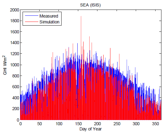
At two locations with three-minute irradiance data, Salt Lake City, UT and Seattle, WA, comparison between simulations and measurements showed significant discrepancies across the distribution’s range. At Salt Lake City, UT, the simulation overestimates the occurrence of high GHI; at Seattle, WA, the simulation underestimates the occurrence of higher values of GHI. Distributions of GHI from each season showed the same trends. These two sites are distinguished from other sites by their distance from any location used to parameterize the simulation. The time series of GHI from simulation and measurement are compared in figures on the right (no measurements are available until February 23, 2010). Investigations by NREL^[7] indicated that the disagreement between simulations and measurements arises from disagreement between the hourly values for GHI obtained from satellite data^[2] and the hourly, measured values for GHI. The simulation uses satellite data to set an hourly target value for the clear-sky index. Testing by NREL confirms that the stochastic simulation methods produce one-minute time series of clear-sky index which maintain these target values. Consequently, the likely explanation for the disagreement between simulated and measured one-minute GHI is that the hourly satellite estimates of GHI do not agree with the GHI measured on the ground.

Locations with Hourly Average GHI Data

We compared simulated GHI with measurements at a number of locations where only hourly averaged measurements are available. At these locations measured GHI is reported as the average over each preceding hour. We averaged the simulated time-series of irradiance over one hour blocks to obtain comparable values.

Distributions of simulated and measured hourly average GHI are compared in figures on the right. At each location, the shape of the distributions of simulated GHI closely follows that of measured GHI, indicating that the simulation is representing relative levels of GHI at appropriate frequencies. However, at many of these locations, we observed a slight bias towards higher GHI values. The bias varied through the year by season, although the variation in bias by season was not consistent among the sites. We have not identified the cause of this bias, which is small enough that it seems unlikely to be important to the use of the simulations in the WWSIS study. Possible explanations include: a systematic error in the estimation of GHI from satellite data (although it would be surprising for this error to be confined within Arizona); systematic error in measuring or reporting GHI from the AZMET network^[8]; or an undetected software error in our calculation of averages of the simulation results.

Comparison of Rates of Change in GHI

We compared distributions of rates of change in GHI between simulated and measured time series for sites for which subhourly (i.e., one-minute or three-minute) GHI measurements are available. We expressed all changes as differences over one minute intervals, linearly interpolating between values of three-minute time series. We filtered out changes (increases or decreases) of less than 10 W/m²per minute to exclude dark periods and periods of time with relatively stable irradiance conditions.

Agreement between simulated and measured rates of change provides confidence that ramps (i.e., changes) in power are represented in the WWSIS simulations with appropriate magnitudes and at appropriate frequencies. If larger ramps occur in simulation results more frequently than are observed in data, then the effects of variable generation sources on load-following and regulating reserves would be overstated, and would cause the consequent costs to be overstated.

Rates of change in GHI at a point do not directly correspond to rates of change in power output because output is generally proportional to the spatial average of plane-of-array irradiance over the plant’s area^[9]. Various methods have been proposed to estimate spatial average irradiance from a time series of point irradiance, including time-averaging^[10][11], applying a filter^[12], and modifying amplitudes of a wavelet transform^[13]. For WWSIS, power calculations involved first smoothing the time series of irradiance using a filter^[12]; the smoothing algorithm is further considered here. We examined both unsmoothed irradiance (i.e., representing irradiance a point) as well as smoothed irradiance that represents spatial average irradiance over typical plant areas.

At one-minute time scales and when not smoothed to represent spatial averages over PV plant areas, we found the simulations generally overstate variability in GHI. However, when smoothed over PV plant areas, the simulation time series compare favorably with smoothed time series of measured GHI. Overall, we view the relatively close agreement between distributions of changes in smoothed GHI time series as evidence that changes in time series of GHI occur with appropriate frequencies. Consequently, we expect that variability in the power output of non-concentrating PV systems will be appropriate for the objectives of the WWSIS study. Variability in power output for concentrating PV systems is discussed here.

Rates of Change in Unsmoothed GHI

Figure on the right illustrates how distributions of changes in GHI are compared between simulations and measurements. The CDFs of per-minute changes in GHI show that, at the University of Las Vegas, NV site, the simulations exhibit more frequent large changes than are evident in measurements. Comparison of percentiles of the distribution of changes illustrates the increase in the magnitude of changes. For example, in the measurements, the greatest 1% of changes (that exceed 10 W/m² per minute) are 300 W/m2 or greater, whereas in the simulations, the greatest 1% of changes are 420 W/m² or greater.

We observe similar results at most other locations, i.e., the simulation results show more variability in GHI than do measurements. We note that changes in either simulated or observed GHI are smaller in magnitude at the four sites having three-minute data than at sites with one-minute data, because the changes are expressed as per-minute ramps in three-minute averages and the time-averaging inherently smoothes the irradiance time series.

However, there are exceptions. At two locations, the distributions of changes in simulated GHI closely match the distributions of changes in measured GHI. Additionally, the variability of simulated GHI is less than that of measured GHI at two other locations: Hanford, CA and Seattle, WA. These latter two locations are both likely influenced by marine climate which may cause variability in GHI which is not represented in the data used to parameterize the distributions of clear-sky index used in the simulation.

Rates of Change in Smoothed Irradiance

We applied the filter used in the WWSIS analysis to smooth GHI time series for locations where one-minute GHI measurements are available. The filter is designed to operate at one-minute time-scales, and at locations with either three-minute or hourly average GHI data, we were unwilling to interpolate between measured values in order to apply the filter. Comparison of changes in smoothed GHI between measured and simulated time series at 15 of 28 locations should be informative of results at the remaining locations.

Figure on the right compares percentiles of the distributions of changes in GHI, measured vs. simulated, for unsmoothed (i.e., point) time series as well as time series smoothed to represent average GHI over solar plants of increasing size: 50MW (1.2 km²); 100MW (2.4 km²); and 200MW (5.2 km²). We observe that the tendency for simulated GHI to overstate the frequency of large changes is significantly reduced by smoothing, although a slight bias towards more frequent large changes remains. Similar effects of smoothing are observed at most but not all other locations examined. At some locations, remarkable agreement between measured and simulated distributions is observed (e.g., at Nevada Power Clark Station). At a few other locations, however, where the distributions of changes in point GHI agreed, the smoothing acts to understate the frequency of large changes in GHI (e.g., Sacramento, CA).

Calculation of Clear-sky Index Values

The clear-sky irradiance is the estimated irradiance incident at the ground (in W/m²) if skies are clear. The clear-sky index is irradiance divided by the clear-sky irradiance. Clear-sky indices are often used to compare irradiance between locations and times because the index removes diurnal and annual variation due to the earth’s rotation and orbit. For the WWSIS simulations, distributions of clear-sky index derived from measured data are used to parameterize the downscaling algorithm that generates one-minute irradiance time series from spatial average values^[3].

Clear-sky irradiance was estimated for the WWSIS study using the Bird clear-sky model^[14]. This model requires a number of inputs that, in theory, are calibrated from measured data, one of which is an estimated broadband aerosol optical depth (broadband turbidity). For the WWSIS, the clear-sky model was calibrated^[3] by visually identifying a few clear days in the measured irradiance data used to calibrate the simulation. For each hour of these days, the clear-sky model was fit to measured GHI by adjusting the aerosol optical depth value for each hour. The fitted values of aerosol optical depth were propagated to days earlier and later than each clear day to create an initial year-long time series of aerosol optical depth at hourly time steps. The initial time series was then smoothed to arrive at a final time series without abrupt changes in the aerosol optical depth values. Finally, clear-sky GHI was computed using the final time series in the Bird clear-sky model.

Clear-sky index values were calculated by dividing GHI by the clear-sky GHI. Because clearsky GHI may be very small in magnitude for brief times at early and late hours, clear-sky index can greatly exceed 1 when computed in this manner. To remove these artificially large values, clear-sky index values greater than 1.2 were replaced by 0.

Comparison of Clear-sky Index Values

We computed and compared correlations between time-series of clear-sky index at different sites, as a function of the distance between sites. We examined correlations between clear-sky index time series rather than between GHI time series so as to remove the predictable diurnal effects, which would artificially inflate correlation coefficients. Agreement between simulated and measured clear-sky index values, and in particular, consistent correlations as a function of distance between sites, provides confidence that appropriate spatial correlations in power levels at different sites are represented in the WWSIS simulations.

Correlation is an aggregate measure of agreement between time series. The same value for the correlation coefficient can be obtained from pairs of time series with substantially different behavior. To ensure that similar correlation coefficients indicate similar time series, we also compared joint distributions of clear-sky index for pairs of sites and CDFs of clear-sky index, between simulated and measured time series. Because the same clear-sky model is used to calculate clear-sky index values from GHI for both simulated and measured irradiance, any bias in simulated GHI (relative to measured GHI) will also be reflected in the comparison of clearsky index values.

Correlation is calculated by considering only hours between 10am and 4pm (local time) at one site and the concurrent values at the second site (which may be one hour earlier or later in local time due to different time zones). Further, from this data set we excluded any times at which the clear-sky index is zero or when the index exceeds 1.2 (we view values exceeding 1.2 as erroneous as they likely result from the poor values for clear-sky irradiance given by the clearsky model during early morning and late afternoon hours). We considered correlations between the annual time series as well as for two-week periods in each season.

Generally we found good agreement between correlation coefficients for simulated and measured time series. Joint distributions of clear-sky index for pairs of sites also compared favorably, as did CDFs of clear-sky index for individual sites, although the simulations showed a tendency towards more variability in clear-sky index than is evident in the measurements. These successful comparisons provide confidence that the simulation results generally reflect spatial correlations in power levels that are implied by measured irradiance. The greater variability in distributions of simulated clear-sky index as compared to distributions of measurements indicates that simulated irradiance conditions are more likely to change independently between locations than in measurements, suggesting that overall, the variability in aggregate power over many sites may be somewhat understated.

Sites with Hourly Average GHI

Figure on the right shows correlation as a function of distance between locations, for locations with only hourly average GHI data, for the simulation year. Values labeled as ‘measured’ indicate correlations between measured time series at two different locations; values labeled as ‘simulated’ are correlations between simulated time series. The exponentially decaying relationship between correlation and distance has been observed and discussed in other analyses (e.g.,^[13][15]). The figure shows remarkable agreement between the correlations for the measured and simulated data sets.

We also examined the joint distributions of clear-sky index for pairs of sites, by means of scatterplots of the time series of measured clear-sky index and the corresponding time series of simulated clear-sky index. To aid in comparing between scatterplots, marginal histograms were added to the plots, using the same bins on each axis and in each plot.

Figure on the right (total of 3,939 points) and the figure bellow (total of 4,132 points) compare measured and simulated hourly average clear-sky index (i.e., the clear-sky index calculated by dividing the hourly average of irradiance by the hourly average of clear-sky irradiance), respectively, between Bonita AZ (site 20) and Buckeye AZ (site 21), which are 172 miles apart. The cluster of points with common clear-sky values between 0.9 and 1.2 indicate that weather conditions are frequently clear at both sites. The horizontal and vertical bands around a clear-sky value of 1.0 on one axis indicate periods of time when the weather is clear at one site, but variable at the other. The scattered points in the remainder of the plot indicate periods when variable weather occurs at both sites. The correlation coefficient between measured time series is 0.39, and between simulated time series, 0.36. Visual comparison of figures on the right show that the simulation generally reproduces the joint distribution of clear-sky index for these two locations, although the clear-sky index values are somewhat more broadly distributed than the measured values (as indicated by the thicker clump in the upper right corner, and the broader width of the horizontal and vertical bands).

The simulated clear-sky index values for sites with hourly average GHI are generally greater than those for measured clear-sky index values; figure on the right illustrates the differences for the Bonita, AZ location (site 20). The greater values of clear-sky index are consistent with observing higher simulated GHI values at sites with only hourly data and result from the same underlying cause, which we have not identified.

Figure on the right (total of 2,029 points) and the figure bellow (total of 2,476 points) compare measured and simulated hourly average clear-sky index, respectively, between Phoenix Encanto (site 26) and Phoenix Greenway AZ (site 27), which are 10 miles apart. The relative proximity of these sites cause the data to cluster about a 1:1 line, indicating that weather is frequently similar at both sites. The limited scatter away from the 1:1 line indicates the relatively low potential for hourly conditions to differ between the two sites. The correlation coefficient between measured time series is 0.87, and between simulated time series, 0.81. Comparison of figures on the right shows that the simulation results in somewhat greater disparity in clear-sky values between these sites than is observed in the data.

We observed similar comparisons of clear-sky index between all other pairs of sites with only hourly data (the numerous figures are omitted from this report). The joint distribution of clearsky index in the simulations is generally similar to that observed in the data, although the simulation results in more scatter between each pair of sites.

Clear-sky index correlations and scatterplots, when restricted to two-week periods in each season, compared similarly among sites.

Sites with Subhourly GHI

Figure on the right shows correlation as a function of distance for sites with either one- or three-minute GHI data. Good agreement between measured and simulated time series is evident.

For pairs of sites with subhourly GHI data, we compared joint distributions of hourly-average clear-sky index rather than values at one- or three-minute time steps, because there is no reason to expect that either data or simulations at fine time scales would be comparable. We averaged available GHI data within each hour of the year and divided by the hourly average clear-sky irradiance. To display the joint distribution of hourly average clear-sky index, we considered only hours between 10am and 4pm (local time) at one site, and the concurrent values at the second site (which may be one hour earlier or later in local time due to time zone effects). We also excluded times at which the hourly average clear-sky index is zero or when the index exceeds 1.2 (we view values exceeding 1.2 as erroneous as they likely result from the poor values for clear-sky irradiance given by the clear-sky model during early morning and late afternoon hours).

We found acceptable agreement between the joint distributions of hourly average clear-sky index between measured data and simulations. At some locations, the joint distributions are in close agreement − for example, figures on the right display measured and simulated, respectively, joint distributions for two sites that are 185 miles apart. At other locations, the scatterplots appear different for measured and simulated data. However, in our judgment, differences between measured and simulated joint distributions arise primarily from different sample sizes rather than from a different representation of the spatial correlation between the two sites. For example, there are fewer points (860) in the plot of measured data than in the simulated results because data for Cedar City, UT, are available for approximately half of 2010, whereas simulation results are provided for all hours. In most cases where joint distributions appear different, the differences can be explained, and accepted, after comparing the marginal distributions between measured and simulated clear-sky index at the same site.

Comparison of Changes in Clear-sky Index Values

We calculated correlations between time series of changes in clear-sky index and compared correlation coefficients as a function of distance between sites. Agreement between the sets of correlation coefficients confirms that changes in irradiance (independent of diurnal or annual sun position effects) are represented in the simulation results with appropriate spatial correlation.

We performed the calculations only for sites with hourly or one-minute GHI data. We filtered the annual time series of clear-sky index values to retain only those values greater than 0 and between 10am and 4pm at one location and paired the result with concurrent values at the second location. We differenced of the resulting time series without removing differences between nonadjacent time steps (e.g., between the last time on one day and the first time on the next). We filtered the simulated time series to retain clear-sky values only at the same times as were retained for measured data.

Figure on the right shows correlation coefficients obtained for pairs of sites with only hourly data; Figure on the right displays results for sites with one-minute data. Acceptable agreement between measured data and simulation results are evident at both time scales. A slight tendency toward greater correlation is evident in the simulation results at one-minute time scales; however, for all distances the correlation coefficients are low enough that a slight bias towards more spatially correlated time series is unimportant.

The results in these figures agree quite well with correlations calculated from other data sets (compare with^[15]).

We confirmed that, over the course of a year, changes in clear-sky index generally agreed between measurements and simulations at each site, by visually examining time-series plots. We also compared scatterplots of changes in measured clear-sky index at pairs of sites, with scatterplots of the corresponding time-series of changes in simulated clearsky index. Figures on the right compare changes in measured and simulated hourly clearsky index (i.e., the clear-sky index calculated from separate hourly averages of irradiance and clear-sky irradiance), respectively, between Bonita AZ (site 20) and Buckeye AZ (site 21), which are 172 miles apart. Points cluster near the center of the plot (around zero change at both sites) because weather conditions are frequently clear at both sites concurrently. The horizontal and vertical bands at values of zero change indicate periods of time when the weather is clear at one site, but variable at the other. The scattered points in the remainder of the plot indicate periods when variable weather occurs at both sites. The correlation coefficient between measured time series of changes is 0.08, and between simulated time series, 0.09. Comparison of figures on the right shows that the simulation generally reproduces the joint distribution of changes in measured clear-sky index for these two locations, although the changes in the simulated clearsky index are more clustered in the center and the central cluster is somewhat more broad (as indicated by the thicker clump in the upper right corner, and the broader width of the horizontal and vertical bands) than the central cluster for the changes in measured clear-sky index. These differences indicate that small changes in hourly clear-sky index occur more frequently in the simulations than in measurements, and that large changes occur less frequently in simulations. However, the differences in these distributions are minor, as illustrated by figure on the right.

Figures on the right compare changes in measured and simulated hourly clear-sky index, respectively, between Phoenix Encanto (site 26) and Phoenix Greenway AZ (site 27), which are 10 miles apart. The relative proximity of these sites cause the data to cluster about a 1:1 line, indicating that irradiance at both sites is likely to change in concert. The degree of scatter away from the 1:1 line indicates the potential for different changes in clear-sky index at the two sites. The correlation coefficient between measured time series is 0.57, and between simulated time series, 0.42. Comparison of figures on the right shows that the simulation overstates somewhat the occurrence of small, uncorrelated changes at the two sites, and understates somewhat the occurrence of large, concurrent changes.

We examined changes in clear-sky index between all other pairs of sites with only hourly data (the numerous figures are omitted from this report). The joint distributions of clear-sky index in the simulations are generally similar to those observed in the data, although the simulation results in more scatter between each pair of sites.

Clear-sky index correlations and scatterplots, when restricted to two-week periods in each season, compared similarly among sites.

Comparison of Simulated DNI

For flate-plate PV systems, power from an array is closely correlated with spatially-averaged plane of array irradiance^[9]. The WWSIS study considers both flat-plate PV and concentrating PV (CPV) power systems, for which power output is more closely correlated with DNI than with GHI. To inform judgment about the suitability of power calculated for CPV systems, we examined the methods used to estimate DNI, and compared CDFs of simulated DNI and distributions of ramps in DNI to measurements.

Overall, we found that the simulated DNI is generally lower in magnitude than the measured DNI. Differences in level of DNI are on the order of 10%. When not smoothed to represent spatial averages over PV plant areas, we found the simulations generally overstate variability in DNI. However, when smoothed over PV plant areas, the simulation time series compare favorably with smoothed time series of measured irradiance. Overall, we conclude that changes in the time series of DNI occur with frequencies comparable to those observed in measurements, and thus changes in power output for CPV systems are likely to be appropriate for their use in the WWSIS study.

Estimation of Irradiance Components

For the WWSIS simulations, components of irradiance were estimated as spatial averages over each plant’s area, rather than being estimated first at points and then spatially-averaged. Instantaneous, spatially aggregated values of DHI and DNI are available in conjunction with the satellite imagery from SolarAnywhere™. These values were linearly interpolated in time and space to obtain a one-minute time series of baseline DHI at each plant location. Next, simulated one-minute GHI was spatially averaged over each plant and compared to a clear-sky model for GHI. When spatially-averaged GHI exceeded the clear-sky irradiance, the excess irradiance was regarded as the result of cloud enhancement (e.g.,^[5],^[6]) and was added to the baseline DHI. Finally, DNI was estimated by subtracting DHI from GHI and dividing by the cosine of the solar zenith angle to translate from a horizontal plane (for GHI) to a plane normal to the line between the earth and sun^[16]. The calculation can be summarized as

\(\overline{DHI}(t) = DHI_{base}(t)+max\left (\overline{GHI}(t)-CSky(t),0\right )\) \(\overline{DNI}(t) = \cfrac{\overline{GHI}(t)-\overline{DHI}(t)}{cos\left (z(t)\right )}\)

where the overline indicates a spatial average and z (t ) is the solar zenith angle.

To our knowledge this method of separating GHI into components is novel. However, we are unaware of other studies where an hourly time series for an irradiance component has been downscaled to a one-minute time series, so we do not view the WWSIS simulation approach as departing from precedent. An alternate approach would be to employ a model, such as the DISC model^[17], which separates GHI into one or both components. However, available models require calibrated parameters, such as atmospheric turbidity, or use empirical relations developed from historical data (e.g., as is the case with the DISC model), which may not be available or appropriate for the region and period of interest.

Comparison of DNI to Measurements

Sufficient measured DNI is available at ten of the locations used for validation. DNI measurements are also available at Sites 14 and 16; however, because simulated GHI does not compare favorably with measured GHI at these locations, comparison of DNI is not expected to be favorable. All locations with DNI measurements have either one-minute or three-minute data.

For comparison of CDFs of DNI, we filtered the simulated and measured time series of DNI to compare only values exceeding 30 W/m2, in order to exclude dark hours. We found that the WWSIS simulations generally underestimate DNI, although the amount varies among the sites. Figure on the right illustrates the comparison for Site 2. For Site 2, high levels of DNI, which correspond to high levels of power generated from CPV systems, are approximately 10% lower than observed in measurements. The simulation also overestimates DNI when DNI is low, indicating that the range of power (high level minus low level) from simulated CPV systems will be less than indicated by available data.

For comparison of CDFs of changes in DNI, we filtered the time series of one-minute changes DNI to exclude changes less than 10 W/m2 per minute, to focus on ramps in DNI of interest, and also excluded changes greater than 1000 W/m2 per minute, to remove any unreasonably large ramps from the statistical comparison. We found that, at many sites, the largest changes in DNI occur more frequently in the simulation results than in the measurements. However, these comparisons are between measurements of DNI at a point, and simulations of DNI spatially averaged over the area of a plant. Earlier, we observed that differences in CDFs of ramps in GHI were reduced when time series were smoothed to represent spatial averages over plant area. We found that applying the smoothing algorithm to DNI mitigated differences between the CDFs of changes in DNI in a similar manner. Figure on the right illustrates the effects of smoothing at the Solar Radiation Research Laboratory site; results for other sites are shown in figures on the right. For some sites, changes in smoothed DNI agree well between simulations and measurements. For other sites, where the initial comparison of changes in DNI was more favorable, the largest ramps in smoothed DNI were lower in simulations than in measurements.

The observed differences between simulated and measured DNI are likely to understate the contribution of CPV systems to aggregate power in the WWSIS study. As a consequence, the effects of variability in power output from the largest CPV plants may be somewhat understated.

Review of Power Calculations

References

- ↑ Sandia, Validation of Simulated Irradiance and Power for the Western Wind and Solar Integration Study, Phase II, October 2012, [Online]. Available: http://energy.sandia.gov/wp/wp-content/gallery/uploads/2012_Hansen_WWSIS_irradiance_sim_validation_final.pdf. [Accessed April 2014].
- ↑ 2.0 2.1 Clean Power Research, LLC. SolarAnywhere®. Retrieved from https://www.solaranywhere.com/Public/About.aspx, June 2012
- ↑ 3.0 3.1 3.2 3.3 Hummon, M., M. Sengupta, K. Orwig, Sub-hour Irradiance Data Research and Synthesis Algorithm, NREL/TP-6A20-54518, National Renewable Energy Laboratory, forthcoming
- ↑ National Renewable Energy Laboratory (NREL). Measurement and Instrumentation Data Center (MIDC). Retrieved from http://www.nrel.gov/midc/, June 2012
- ↑ 5.0 5.1 Nils H. Schade, Andreas Macke, H. Sandmann, and C. Stick, Enhanced solar global irradiance during cloudy sky conditions, Meteorologishe Zietschrift, Vol. 16, pp. 295-303, June 2007
- ↑ 6.0 6.1 Yordanov, G. H., O. Midtgård, T. O. Saetre, H. K. Nielsen, L. E. Norum, Over-Irradiance (Cloud Enhancement) Events at High Latitudes, Proc. of the 38th IEEE Photovoltaic Specialist Conference, Austin TX, June 2012
- ↑ Private communication from M. Hummon, National Renewable Energy Laboratory, July 2012
- ↑ The University of Arizona. AZMET: The Arizona Meteorological Network. Retrieved from http://ag.arizona.edu/azmet/, June 2012
- ↑ 9.0 9.1 Kuszmaul, S., A. Ellis, J. Stein, L. Johnson, Lanai High-Density Irradiance Sensor Network for Characterizing Solar Resource Variability of MW-Scale PV System, Proc. of the 35th IEEE Photovoltaic Specialist Conference, Honolulu, HI, 2010
- ↑ 10.0 10.1 Longhetto, A., G. Elisei, C. Giraud, Effect of correlations in time and spatial extent on performance of very large solar conversion systems, Solar Energy 43(2), 77-84, 1989
- ↑ Hansen, C.W., J. S. Stein, A. Ellis, Simulation of One-Minute Power Output from Utility-Scale Photovoltaic Generation Systems, SAND Report 2011-5529, Sandia National Laboratories, Albuquerque, NM, 2011
- ↑ 12.0 12.1 12.2 Marcos, J., L. Marroyo, E. Lorenzo, D. Alvira, and E. Izco, From Irradiance to Output Power Fluctuations: the PV Plant as a Low-Pass Filter, Prog. In Photovoltaics: Research and Applications 19, 505-510, 2011
- ↑ 13.0 13.1 13.2 Lave, M., J. Kleissl, and E. Arias-Castro, 2011. High-frequency irradiance fluctuations and geographic smoothing. Solar Energy 86(8), 2190-2199, 2012
- ↑ Bird, R. E., and R. L. Hulstrom, Simplified Clear Sky Model for Direct and Diffuse Insolation on Horizontal Surfaces, Technical Report No. SERI/TR-642-761, Golden, CO: Solar Energy Research Institute, 1981
- ↑ 15.0 15.1 Mills, A. and R. Wiser, Geographic Diversity for Short-Term Variability of Solar Power, LBNL-3884E, Lawrence Berkeley National Laboratory, Berkeley, CA, Sept. 2010
- ↑ Handbook of Photovoltaic Science and Engineering, 2nd ed., Eds. A. Luque and S. Hegedus, Wiley, 2011
- ↑ Maxwell, E. L., A Quasi-Physical Model for Converting Hourly Global Horizontal to Direct Normal Insolation. Golden, CO, Solar Energy Research Institute, 1987
- ↑ Hummon, M., J. King, A. Dobos, E. Ibanez, G. Brinkman, D. Lew, Sub-hour Solar Power Data for Western Wind and Solar Integration Study (WWSIS) II, NREL/TP-6A20-54517, National Renewable Energy Laboratory, forthcoming
- ↑ National Renewable Energy Laboratory (NREL). PVWatts™. Retrieved from http://www.nrel.gov/rredc/pvwatts/, June 2012